Overview
This assignment consists of two parts. In the first, you'll get to
implement Monte Carlo sampling techniques that warp an initially
uniform distribution into a number of different target distributions.
Note that all work you do in this assignment will serve as building
blocks in later assignments when we apply Monte Carlo integration to
render images. In particular, assignments 4 and 5 will build on this
functionality to create material models and light sources suitable for
photorealistic rendering.
In the second part, you will implement two very basic rendering
algorithms: the first algorithm is fully deterministic and renders a
scene illuminated by a single point lights. The second is a
stochastic rendering algorithm known as Ambient Occlusion,
which assumes that the scene is uniformly illuminated from all
directions.
As usual, begin by importing the latest base code updates into your
repository by running
$ git pull upstream main
If there were any concurrent changes to the same file, you
may have to perform a merge (see the git tutorials under
"Preliminaries" for more information).
For this homework, we will be using the scene scenes/pa2/ajax-ao.xml and scenes/pa2/ajax-simple.xml.
This scene references the 3D scan of a bust that is fairly large (~500K triangles). Due to
its size, the actual mesh is not part of the repository and can be downloaded
here.
Warning: For this same reason, we ask you not to commit the file to
your repository. To make sure this doesn't happen, you can add the file
to your repository's .gitignore file (located at the root).
Part 1: Monte Carlo Sampling (60 pts)
In this exercise you will generate sample points on various domains:
the plane, disks, spheres, and hemispheres. The base code has been
extended with an interactive visualization and testing tool to make
working with point sets as intuitive as possible.
After pulling the latest updates and recompiling,
you should see an executable named warptest. Run this
executable to launch the interactive warping tool, which allows you to
visualize the behavior of different warping functions given a range of
input point sets (independent, grid, and stratified). Up to now, we
only discussed uniform random variables which correspond to the
"independent" type, and you need not concern yourself with the others
for now.
Part 1 is split into several subsections; in each case, you are asked to
implement a distribution function and a matching sample warping scheme.
It is crucial that both are consistent with respect to each
other (i.e. that warped samples have exactly the distribution described
by the density function). Significant errors can arise if inconsistent
warpings are used for Monte Carlo integration. The
warptest tool provided by us implements a \(\chi^2\) test to
ensure that this consistency requirement is indeed satisfied.
Note that passing the test does not generally imply that your
implementation is correct—for instance, the test may not have enough
"evidence" to generate a failure, or potentially the warping function
and the density function are both incorrect in the same manner. Use
your judgment and don't rely on this test alone.
Note: the continuous integration will now automatically run
the warptest tool as well as compile your code. This means that
until all features have been implemented, you will likely see a
"failed build" on Github Actions.
We ask you to not modify the run_tests.py
script.
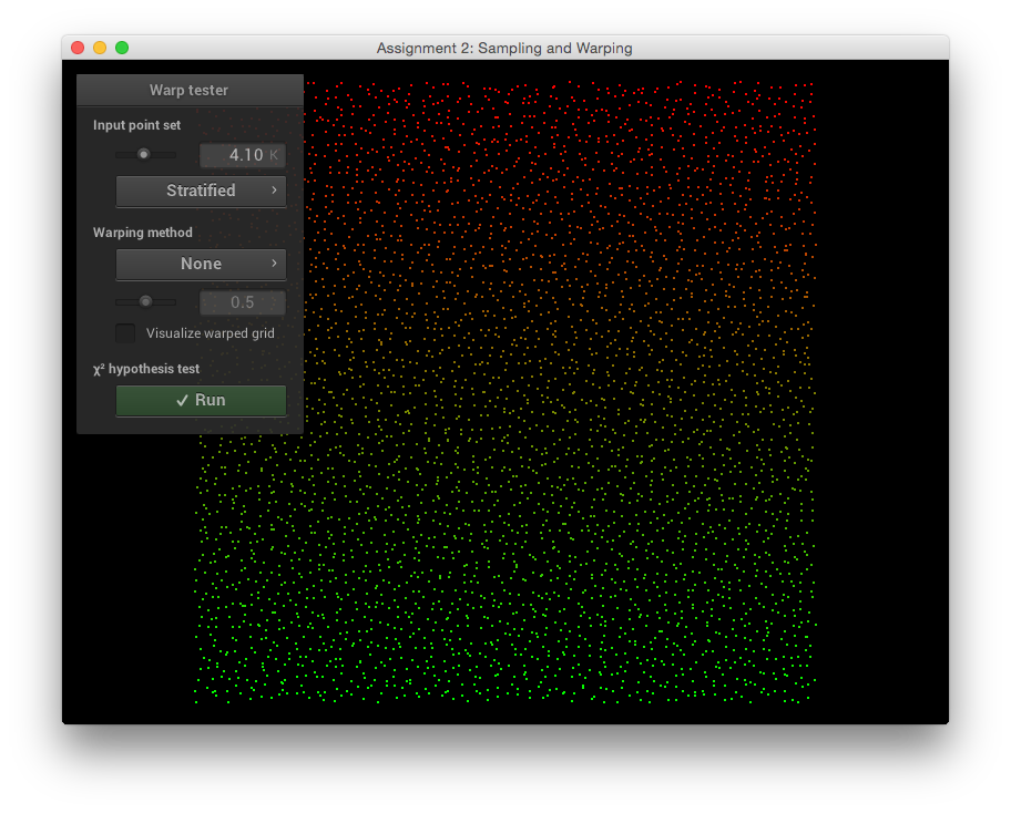
The input point set (stratified samples passed through a "no-op" warp function)
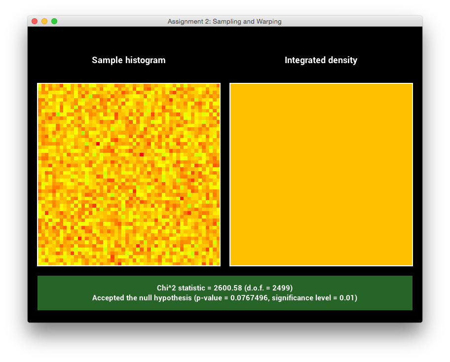
This point set passed the test for uniformity.
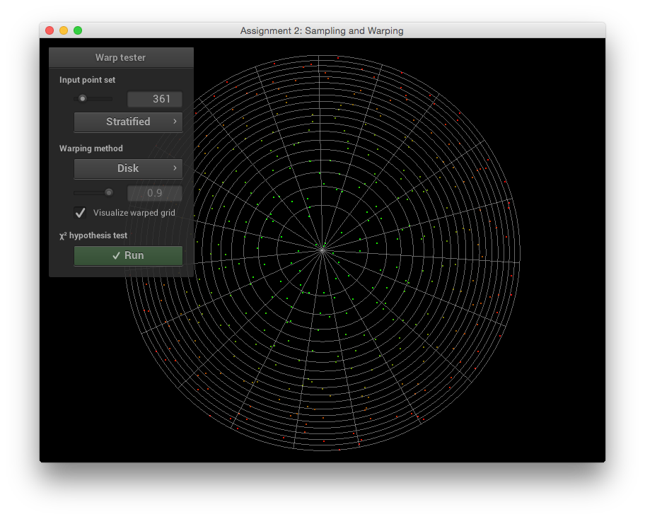
A more interesting case that you will implement
(with a grid visualization of the mapping)
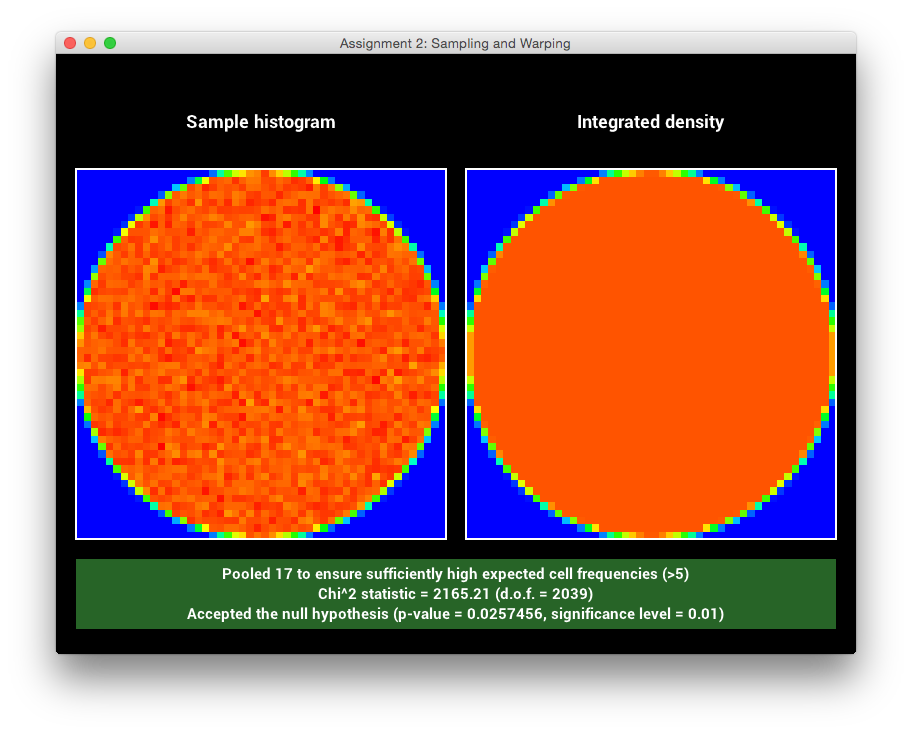
This warping passed the tests as well.
Implement the missing functions in class Warp found in
src/warp.cpp. This class consists of various warp methods that
take as input a 2D point \((s, t) \in [0, 1) \times [0, 1) \) and
return the warped 2D (or 3D) point in the new domain. Each method is
accompanied by another method that returns the probability density with
which a sample was picked. Our default implementations all throw an
exception, which produces an error message in the graphical user
interface of warptest. The slides on the course website
provide a number of useful recipes for warping samples and computing
the densities, and the PBRT textbook also contains considerable
information on this topic that you should feel free to use.
Pass the \(\chi^2\) test for each one of the following sampling techniques and include corresponding screen shots in your report:
-
Warp::squareToTent and Warp::squareToTentPdf (15 Points)
Implement a method that transforms uniformly distributed 2D
points on the unit square into the 2D "tent" distribution,
which has the following form:
\[
p(x, y)=p_1(x)\,p_1(y)\quad\text{and}\quad
p_1(t) = \begin{cases}
1-|t|, & -1\le t\le 1\\
0,&\text{otherwise}\\
\end{cases}
\]
Note that this distribution is composed of two independent 1D
distributions, which makes this task considerably easier. Follow
the "recipe" discussed in class:
- Compute the CDF \(P_1(t)\) of the 1D distribution \(p_1(t)\)
- Derive the inverse \(P_1^{-1}(t)\)
- Map a random variable \(\xi\) through the inverse \(P_1^{-1}(t)\) from the previous step
Show the details of these steps in your report (either using TeX, or by taking
a photograph of the derivation and embedding the image)
-
Warp::squareToUniformDisk and Warp::squareToUniformDiskPdf (5 Points)
Implement a method that transforms uniformly distributed 2D
points on the unit square into uniformly distributed points on
a planar disk with radius 1 centered at the origin. Next,
implement a probability density function that matches your
warping scheme.
-
Warp::squareToUniformSphere and Warp::squareToUniformSpherePdf (5 Points)
Implement a method that transforms uniformly distributed 2D
points on the unit square into uniformly distributed points on
the unit sphere centered at the origin. Implement a matching
probability density function.
-
Warp::squareToUniformHemisphere and Warp::squareToUniformHemispherePdf (5 Points)
Implement a method that transforms uniformly distributed 2D
points on the unit square into uniformly distributed points on
the unit hemisphere centered at the origin and oriented in
direction \((0, 0, 1)\). Add a matching probability density
function.
-
Warp::squareToCosineHemisphere and Warp::squareToCosineHemispherePdf (5 Points)
Transform your 2D point to a point distributed on the unit
hemisphere with a cosine density function
\[
p(\theta)=\frac{\cos\theta}{\pi},
\]
where \(\theta\) is the
angle between a point on the hemisphere and the north pole.
-
Warp::squareToBeckmann and Warp::squareToBeckmannPdf (25 Points)

The Beckmann distribution plotted for different values of \(\alpha\).
Transform your 2D point to the Beckmann distribution, which will be used to model the probability density of normals on a random rough surface in a later assignment:
\[
D(\theta, \phi) = \underbrace{\frac{1}{2\pi}}_{\text{azimuthal part}}\ \cdot\ \underbrace{\frac{2 e^{\frac{-\tan^2{\theta}}{\alpha^2}}}{\alpha^2 \cos^3 \theta}}_{\text{longitudinal part}}\!\!\!.
\]
Note that this definition is normalized such that it integrates to one over the hemisphere:
\[
\int_{0}^{2\pi}\int_0^{\frac{\pi}{2}} D(\theta, \phi)\sin\theta\,\mathrm{d}\theta\,\mathrm{d}\phi=1.
\]
Complete the function
Warp::squareToBeckmannPdf so that it evaluates \(D\) using the above definition.
The function takes a normalized Cartesian 3D vector \(\omega\) as input, whose components can be interpreted using the following spherical coordinate representations:
\[
\omega=\begin{pmatrix}
\sin\theta\cos\phi\\
\sin\theta\sin\phi\\
\cos\theta
\end{pmatrix}
\]
Take a look
at the methods in the Frame class if you find yourself
evaluating trigonometric functions in the body of Warp::squareToBeckmannPdf.
Having implemented a way to query this distribution, we'll now want to generate points on the sphere that exactly follow the distribution.
Note how the \(D(\theta,\phi)\) is symmetric around the north pole (in other words: its spherical coordinate representation is separable). Sampling can thus be split into two steps:
-
Uniformly sampling the azimuth \(\phi=2\pi\xi_1\) given a uniform variate \(\xi_1\).
-
Mapping a second uniform variate \(\xi_2\) through the inverse CDF of \(D\)'s
longitudinal part to obtain \(\theta\).
Follow these two steps and implement the resulting sampling technique in Warp::squareToBeckmann. Show the details of the necessary steps and derivations in your report. The statistical test implemented in the warptest executable should pass for different values of \(\alpha\).
Hint: You might find integration by substitution useful,
e.g. using the mappings \(x = \cos{\theta}\) and \(\tan^2{\theta} = \frac{1-x^2}{x^2}\).
In addition this identity might come in handy:
\[
\int f'(x) ~ e^{~f(x)}\,\mathrm{d}x = e^{~f(x)} + C\text{, where } C\in\mathbb{R}
\]
Part 2: Two simple rendering algorithms (40 points)
In this part of the homework, you'll implement two basic rendering
algorithms that set the stage for fancier methods investigated later
in the course. For now, both of the methods assume that the object is
composed of a simple white diffuse material that reflects light
uniformly into all directions.
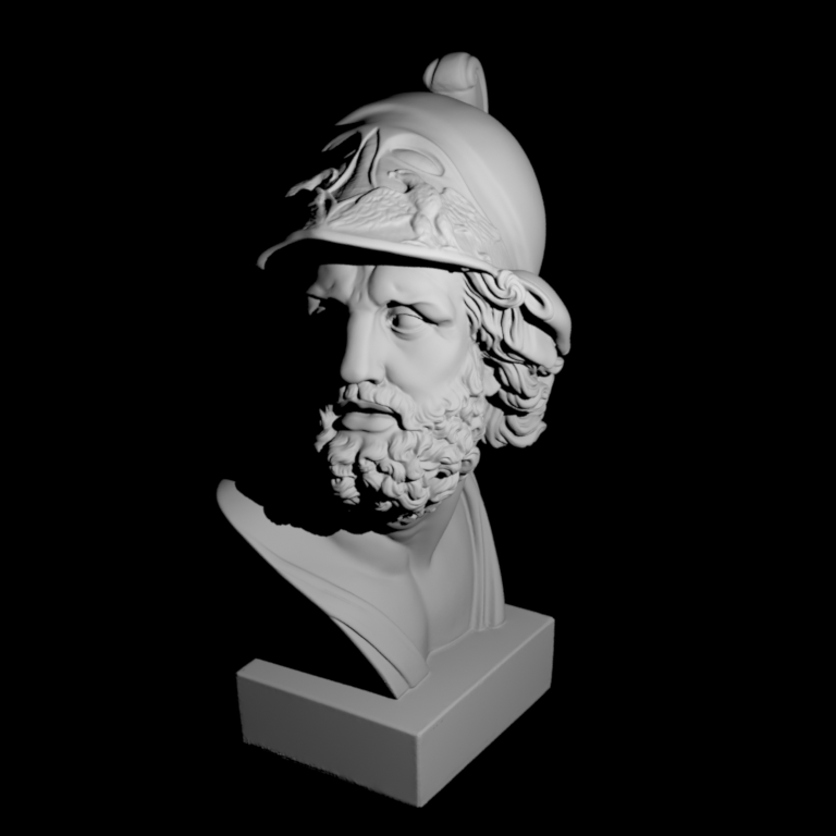
The Ajax bust illuminated by a point light source.
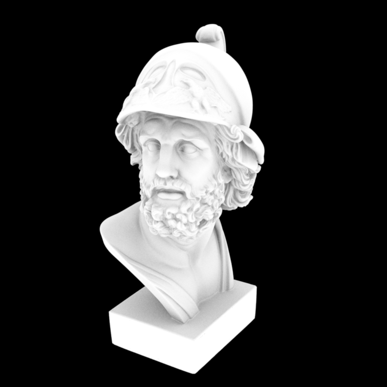
The Ajax bust rendered using Ambient Occlusion.
Part 2.1: Point lights (20 points)
The updated base code includes a new scene scenes/pa2/ajax-simple.xml that instantiates a (currently nonexistent) integrator/rendering algorithm named simple, which simulates a single point
light source located at a 3D position position, and which emits an amount of
energy given by the parameter energy.
<!-- An excerpt from scenes/pa2/ajax-simple.xml: -->
<integrator type="simple">
    <point name="position" value="-20, 40, 20"/>
    <color name="energy" value="3.76e4, 3.76e4, 3.76e4"/>
</integrator>
Your first task will be to create a new Integrator that accepts
these parameters. This should be fairly reminiscent of the normal
integrator from Assignment 1. Take a look at the PropertyList class, which
should be used to extract the two parameters.
Let \(\mathbf{p}\) and \(\mathbf{\Phi}\) denote the position and energy of
the light source, and suppose that \(\mathbf{x}\) is the point being
rendered. Then this integrator should compute the quantity
\[
L(\mathbf{x})=\frac{\Phi}{4\pi^2} \frac{\mathrm{max}(0, \cos\theta)}{\|\mathbf{x}-\mathbf{p}\|^2} V(\mathbf{x}\leftrightarrow\mathbf{p})
\]
where \(\theta\) is the angle between the direction from \(\mathbf{x}\) to \(\mathbf{p}\) and the shading surface normal
(available in Intersection::shFrame::n) at \(\mathbf{x}\)
and
\[
V(\mathbf{x}\leftrightarrow\mathbf{p}):=\begin{cases}
1,&\text{if $\mathbf{x}$ and $\mathbf{p}$ are mutually visible}\\
0,&\text{otherwise}
\end{cases}
\]
is the visibility function, which can be implemented using a shadow ray query.
Intersecting a shadow ray against the scene is generally cheaper since it suffices
to check whether an intersection exists rather than having to find the closest one.
Implement the simple integrator according to this specification and
render the scene scenes/pa2/ajax-simple.xml.
Include a comparison against our reference image in your report.
Part 2.2: Ambient occlusion (20 points)
Ambient occlusion is a rendering technique that assumes that a
(diffuse) surface receives uniform illumination from all directions
(similar to the conditions inside a light
box), and that visibility is the only effect that matters. Some
surface positions will receive less light than others since they are
occluded, hence they will look darker. Formally, the quantity computed
by ambient occlusion is defined as
\[
L(\mathbf{x})=\int_{H^2(\mathbf{x})}V(\mathbf{x}, \mathbf{x}+\alpha\omega_i)\,\frac{\cos\theta}{\pi}\,\mathrm{d}\omega_i
\]
which is an integral over the upper hemisphere centered at the point
\(\mathbf{x}\). The variable \(\theta\) refers to the angle between the direction \(\omega_i\)
and the shading normal at \(\mathbf{x}\). The ad-hoc variable \(\alpha\) adjusts
how far-reaching the effects of occlusion are.
Note that this situation—sampling points on the hemisphere with a cosine weight—exactly corresponds
to one of the warping functions you implemented in part 1, specifically squareToCosineHemisphere. Use this function to sample a point on the hemisphere and then check for visibility
using a shadow ray query. You can assume that occlusion is a global effect (i.e. \(\alpha=\infty\)).
One potential gotcha is that the samples produced by squareToCosineHemisphere lie in the reference hemisphere and need to be oriented according to the surface at \(\mathbf{x}\). Take a look at the Frame class, which is intended to facilitate this.
Implement the ambient occlusion (ao) integrator and render the scene scenes/ajax/ajax-ao.xml.
Include a comparison against our reference image in your report.